Level 400, episode 7. In RAG explained then built in .NET, we called SearchAsync(queryVector, top: 5) and — magic — the five neighbors came up. An architect distrusts magic: how do you find the 5 nearest among ten million vectors, in 20 milliseconds?
Answer: you don’t find the real nearest. You cheat intelligently. Today: the internals of a vector index (HNSW), the trade-off you accept without knowing it, and the layers that turn a demo into a serious search engine. You’ll see: it’s not rocket science.
The wall: exact search doesn’t scale
Naive search is simple: to find a query’s neighbors, you compute its distance to each stored vector, then sort. Over 10,000 chunks, instant. Over 10 million, every query compares 10 million 1,536-dimension vectors — hundreds of milliseconds, even seconds. At scale, exact search (exact k-nearest neighbors) collapses.
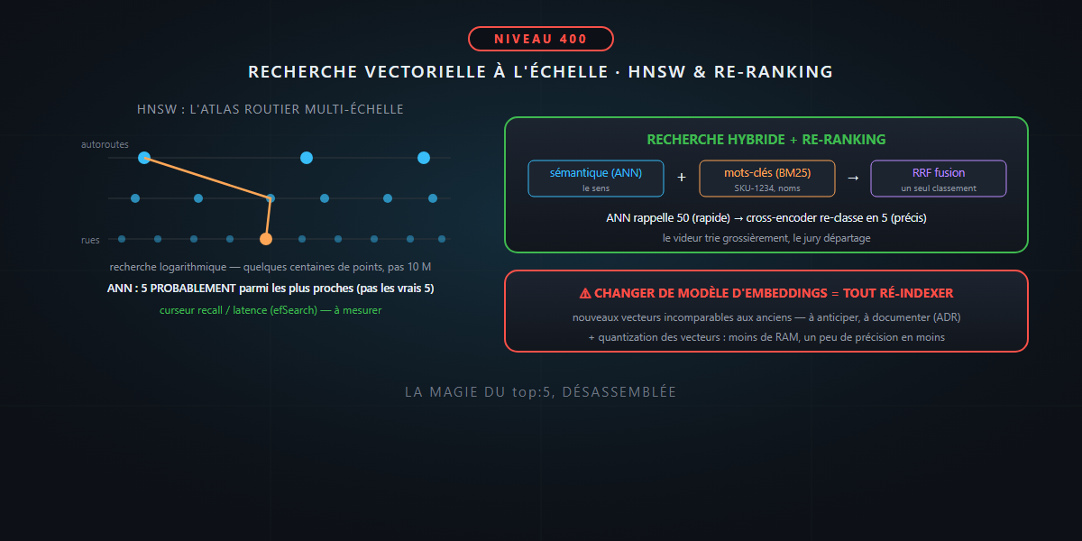
Hence the founding renunciation, and it must be named clearly: you abandon exactness for speed. It’s ANN — Approximate Nearest Neighbors. You no longer look for the true 5 nearest, but 5 very probably among the nearest. That little word, “approximate”, is the key to all of modern vector search — and the parameter you tune without knowing it.
HNSW: the multi-scale road atlas
The dominant algorithm (the one behind most vector databases) is called HNSW — Hierarchical Navigable Small World. The right image is a road atlas with several zoom levels:
- The top layer: the highways. Few nodes, long jumps — you cross the continent of ideas in a few bounds.
- The bottom layers: the streets. Many nodes, short steps — you refine down to the right address.
A query enters at the top, makes big jumps toward the right region, then “descends” layer by layer, refining, like a GPS going from highway to secondary road to street. Result: instead of visiting 10 million points, you visit a few hundred — search time grows logarithmically, not linearly. That’s what makes the top: 5 instant.
And here’s the knob HNSW puts in your hands: the recall/latency trade-off. The search parameter (often efSearch) controls how many paths you explore. Higher = more region covered = better recall (you miss fewer true neighbors) but slower. Lower = faster but you sometimes miss the right one. Tuning a vector database is essentially placing that slider for your tolerance — and it’s measured with a search golden dataset, exactly like at level 300.
Vector quantization: the KV cache has a cousin
Remember: quantization compressed a model’s weights to fit in VRAM. Same idea, different target: ten million 1,536-dimension vectors in 32 bits is heavy — and a vector index’s RAM is expensive. You compress the vectors themselves: scalar quantization (32 → 8 bits, ×4 memory saved) or product quantization (more aggressive). You lose a bit of distance precision, you gain enormous space and speed. The same precision/resources trade-off as everywhere in this series — to be measured, always, on your data.
The two layers that make a real engine
Basic RAG (embed → ANN → prompt) has two blind spots that production reveals fast:
1. Hybrid search. Embeddings capture meaning — but stumble on the exact: a product reference SKU-1234, a rare proper noun, an identifier. Good old keyword (BM25), on the other hand, excels there and fails on meaning. The solution isn’t to choose: it’s to fuse the two rankings. The standard algorithm is RRF (Reciprocal Rank Fusion) — it combines the semantic rank and the lexical rank without having to calibrate heterogeneous scores. Semantic and keyword, the best of both worlds.
2. Re-ranking. ANN is fast but coarse: it compares the query and the chunks separately (each has its vector, computed once). A cross-encoder, on the other hand, reads the query and a chunk together — far more precise, but too slow for ten million. Hence the two-stage pattern, universal in serious engines: ANN recalls 50 plausible candidates (fast), the cross-encoder re-ranks them finely to keep only 5 (precise). The bouncer at the door does the coarse sorting, the jury inside decides — each with its role.
The word of honesty: migrating embeddings hurts
The trap nobody mentions before living it. The day a better embedding model comes out, you can’t just “change the model”: the new vectors aren’t comparable to the old ones (different model = different map of ideas, incompatible coordinates). An embedding migration means re-indexing the entire corpus — costly, slow, and to be done without breaking the live service. The strategies exist (dual indexing, gradual switchover, vector-space versioning), but it’s a heavy operation to anticipate from the design stage, and to record in an ADR. The choice of embedding model is far more binding than it looks.
In summary
- At scale, exact search collapses: you move to ANN (approximate) — 5 probably among the nearest, not the true 5.
- HNSW = a multi-scale road atlas: logarithmic search, with the recall/latency slider (
efSearch) to place and measure. - Vector quantization (cousin of the weights’) trades a bit of precision for a lot of RAM and speed.
- A real engine adds two layers: hybrid search (RRF: semantic + keyword) and re-ranking (cross-encoder refining the top 50 into a top 5).
- And the architect’s trap: changing embedding model = re-indexing everything — to anticipate and document.
“Find the 5 nearest” hid a road atlas, an owned renunciation of exactness, and a bouncer paired with a jury. The magic of top: 5, disassembled. And that, honestly… is not rocket science.